The NEID Queue
Principal Investigators with observing programs in the NEID Queue will be responsible for managing many details of their programs. This user guide describes how PIs, or their collaborators, do that.
For help: If you have difficulties or questions about using the queue, please reach out to the following people for assistance:
- NEID Queue Coordinator, Heidi Schweiker (heidi.schweiker@noirlab.edu)
- NEID Instrument Scientist, Sarah Logsdon (sarah.logsdon@noirlab.edu)
What's New? Here is a list of recent changes to this guide.
The NEID Portal
PIs from all successful proposals will be provided a user account for the NEID Portal, which is accessed using a web browser. PIs will use this portal to specify targets and observing parameters for their programs. Users may have an existing account from a previous semester, in which case the previous program(s) will be visible along with one for the latest semester.
The NEID Portal can be accessed here:
https://wiyn-queuemaster.kpno.noirlab.edu/
Once on the main NEID Portal page, you can login using your email address and password. Once logged in, you will see navigation links at the top of the page, including the Programs link, where you can manage your program.
Overview of NEID Queue Programs
The NEID queue design provides users access to tools to plan, define and monitor a NEID queue observing program. NEID is principally envisioned for use in high-precision radial velocity measurements of exoplanet host stars. Much of the queue planning was done with this purpose in mind. It is hoped that the queue design is also flexible enough to carry out other types of observing programs.
Users' interaction with their queue programs is envisioned as a process that will continue throughout the semester, at least for many users. Users may want to modify the details of their programs to adjust to changing priorities and experience. Those who make an effort to actively monitor their progress and make adjustments may fare better in reaching the full capabilities of NEID.
The NEID queue is one in which observations from multiple users “compete” against each other for telescope time and are scheduled automatically if they score well enough against other observations available at the same time. Through various observational constraints, users may determine when or how often their observations are made available for scheduling (within the physical limits of WIYN and on the nights NEID is scheduled). The priority level of telescope time users attach to a given observation is the principal weight used by the automatic scheduler software to select one observation over another. The availability of a given observation is another important factor determining the likelihood that it gets executed. An observation that is available more often has more chances to win out against the set of competing observations. Other weights will attempt to balance queue time between partners and increase scheduling efficiency and optimize conditions for NEID data.
The NEID queue is still in the process of development as we gain more operational experience. The functioning of the queue software will likely be modified somewhat, even during a semester. NEID queue users are encouraged to provide feedback from their experiences using it and may direct their comments to the NEID queue coordinator and NEID scientist.
Defining a NEID Queue Program
The following describes some terminology and data structures which hold user settings that the queue software uses to execute an observing program. It also describes the steps users should follow to define their queue programs.
Queue users will have proposed a set of targets or described the methods they will use to select targets, if not finalized by the proposal due date. Accepted programs will be given an allocation of observing time and user accounts in a queue database at WIYN. Once logged in, users can start defining their observing program by entering data into the queue database. The steps are:
- Users enter target data, typically by submitting a target ID to query online databases.
- Each target will be reviewed by WIYN staff, who will set its status to "Approved" upon approval (or may contact the PI for more information if necessary).
- Queue users start defining observations based on their targets. Observations specify how targets will get observed and under which conditions. An observation is the schedulable entity in the NEID queue and each execution of the observation is termed a visit.
- Users exert control over their observing program by creating observations and adjusting them over the semester. New targets may also be entered for approval and use in the queue.
Conceptually, the relationship between observations, observation settings, exposures and targets may be understood by describing example observations.
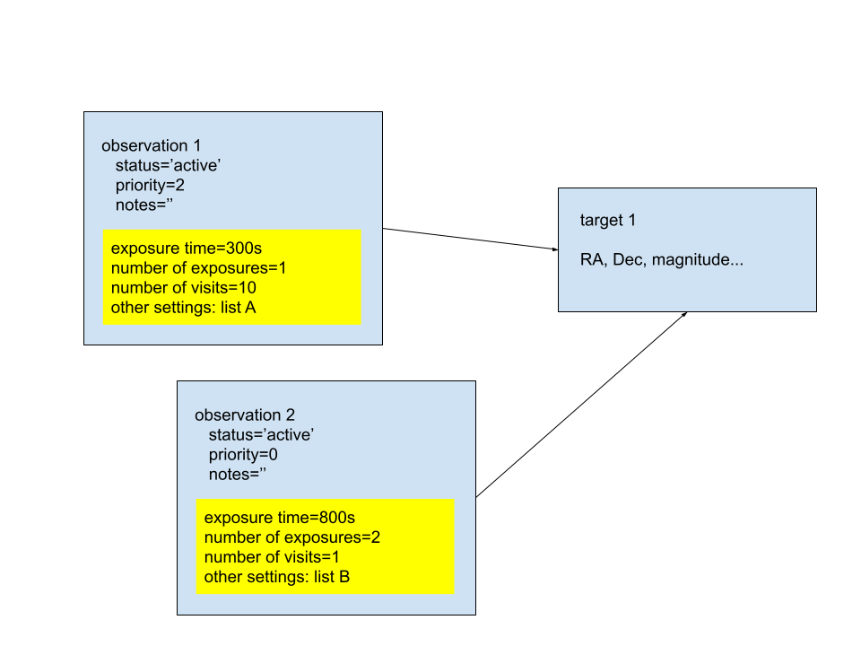
The two observations outlined above define exposures to be taken of one target, an astronomical object, and under what conditions they should be done. Each observation has settings that are user-selectable. For example, the user can set the observation as active or inactive. Active observations are available for scheduling in the queue and inactive observations are unavailable (assuming the observing program has telescope time still available). Other settings include the priority level (which is user-selectable for some programs) and those which control timing or observing conditions (which dictate when an observation is available for scheduling).
There is one target in this example, which is used by both observations. The two observations call for different exposure times and specific numbers of back-to-back exposures to be obtained each time the observation is executed.
Finally, a "visit" describes a single execution of an observation. A single observation may get multiple visits, and this number is requested in the observation settings. However, the number of requested visits is not a guarantee and each visit represents a completion of part of the program, which is charged for the time used.
The details of an existing observation may be edited between visits and will remain the same observation as far as the queue is concerned (e.g., the behavior of an observation may depend on when its last visit occurred). Two different observations may observe the same target, as indicated in the figure, but will be independently scheduled and compete against one another along with other observations in the queue.
Note that the current observation entry software doesn’t permit observations combining more than one target. If that capability is needed for your science, contact the NEID instrument scientist, Sarah Logsdon. A future observation entry tool will have this capacity.
Dates and Times
Note that dates and times used by the NEID queue are expressed as UT or non-timezone values like JD. At WIYN, each night is confined to a single UT date (ie. the earliest sunsets occur at ~ UT 00:22). The timing of some observations might be ideally expressed in terms of BJD, but the NEID queue software uses topocentric or geocentric timing systems. The ability of the NEID queue to start exposures at a specific time is limited by various operational issues. The difference between JD and BJD is less than the precision at which exposure start times can be expected.
Certain values entered by queue users are times, which are sometimes referred to as ‘date-type’ values in this user guide. Most notably these times include the Start and End times along with Time of Phase Zero, all of which are used to define observations. These times refer to UT and may be specified using an ISO format string specifying year, month and day of month (YYYY, MM and DD separated by hyphens) followed by the letter ‘T’ and then hours, minutes and seconds (hh, mm and ss separated by colons):
Fixed vs. SNR-limited Exposure Times
Users have the ability to specify either a traditional fixed exposure time for each observation or a signal-to-noise ratio (SNR) at which they would like to stop each exposure. The latter choice is enabled by NEID’s chromatic exposure meter which gathers a time series of low-resolution spectra in parallel to each science spectrum. The SNR of each exposure is measured in real-time from this exposure meter time series. A SNR-limited exposure is stopped when either the requested SNR is reached or the user-specified maximum exposure time has elapsed (whichever comes first). Users select one of 4 reference wavelengths for measuring the SNR.
For a fixed exposure time the user should set the Exposure Time value, but not set an SNR value.
For a SNR-limited exposure the user must set three values: Exposure Time, SNR and SNR Reference Wavelength. If SNR is set, the Exposure Time value is assumed to be the maximum acceptable exposure time for each exposure.
Defining Targets
The first step toward setting up the observing program is to define targets by entering information in the Target Entry Form. Once completed, the user will submit the target for approval and inclusion in the NEID queue.
Any new target or observation must be entered at least 10 days in advance of when it is expected to be observed. Any edits to existing targets or observations must be completed at least 3 days in advance of expected execution. If a change or addition is needed within these deadlines we will make a reasonable effort to accommodate such requests, but there is no guarantee it can be granted.
Starting Out (please use target query tool if possible)
First, go to the Programs link from your NEID Portal Home Page, select your specific program and then select the All Targets link. This will take you to a list of targets that are part of your program, once you have some defined.
Next, you can add targets and submit them for approval by clicking the green Add Target link at the top of the target list page:

The NEID queue seeks to standardize the use of Gaia DR2 data in its databases (ie. use Gaia DR2 target coordinates, proper motions and magnitudes when possible). Users that enter stellar targets are asked to start by entering a Target ID in the Database Query Tool! This tool defaults to sending the query to Simbad. The primary exception to this rule may be transient targets not found in Simbad or one of the stellar catalogs used by the Query Tool. Read below for instructions on entering these targets.
Widget to run the Target ID Search:

If you wish to check on the type of target ID that is searchable using Simbad, you may test it from Simbad’s identifier query at Strasbourg or its CfA mirror:
http://simbad.u-strasbg.fr/simbad/sim-fid
http://simbad.cfa.harvard.edu/simbad/sim-fid
Users who have targets whose principal source is the TESS Input Catalog (TIC) may enter the TIC ID in the Target Entry Form as “TIC X” where X is an integer. This will query the TIC, then other databases at the coordinates of the TIC ID. Similarly, a target in the Gaia DR2 Catalog may be entered using a string of the form “Gaia DR2 X” where X is an integer.
This tool searches various online databases and catalogs (ie., Simbad, Gaia DR2, Hipparcos and TIC as needed). A successful query will generate a pop-up window listing many values for the target found on-line and ask you to either auto-fill the Target Entry Form with the search results or cancel the action. If the pop-up window lists target IDs, coordinates and some other values, it is presumably a valid entry and the user can choose to auto-fill the form.
Users should not alter the contents of these auto-filled data unless they are given the okay by WIYN staff. This is important to ensure proper handling by the data reduction pipeline and archive.
There are 3 notable exceptions of target entry form fields that users may want to enter manually or edit:
- Alternate Target Name may be used to give a stellar target an additional ID and is needed for non-stellar sources as described below.
- Teff (effective temperature) is the initial input used by the RV data reduction pipeline to select a spectral template for its calculations. However, the pipeline does not require more than a crude estimate of Teff. The values found through the on-line query may not be as accurate as values known to PIs, so this may be edited if you can provide a better value.
- Spectral Type is a secondary alternative to Teff. The pipeline will use Teff when available. PIs may have a better value for Spectral Type than was found using the on-line sources.
When the Query Tool Doesn't Apply (e.g., non-stellar targets)
Users who have non-stellar targets or stars not found by the query tool described above will need to type in coordinates and other information to fully specify the target to the queue database. Such targets should be identified through the Alternate Target ID described below. Please note that if your target was not found through the Query Tool and you’re surprised it isn’t in one of the catalogs listed or known to Simbad, you may have entered the incorrect ID format and it will be helpful if you try again to use the query tool or perhaps the Simbad website to determine a valid ID before trying to re-enter your target.
Alternate Target Names
The Target Entry Form has a field labeled “Alternate Target Name” that can be used for additional target IDs. For most users, this field is optional. For a few, it will be required.
Successful target name searches for stars should automatically fill in one or more Object IDs from the HD, TIC, 2MASS Point Source and Gaia DR2 catalogs in their associated fields on the Target Entry Form. In these cases, users may provide an optional string in the Alternate Target Name field. This string could be a traditional object ID from another catalog, a user's internal management system, or anything else that's useful. It need not be unique. It could be used to describe a class or type of target and may be used in the future for sorting or searches of a target list. This string will be passed to NExScI and might be included in the archive! An alternate object ID should not appear to be deceptive, like an object from a known catalog, but with an incorrect ID.
Users whose target is not found in the target query or is not identifiable in one of the stellar catalog fields are required to enter a unique, useful target ID in the Alternate Target ID field. Whenever possible, this ID should be something in standard use by the astronomical community. The following database sources should be consulted for appropriate IDs:
‘target body’ names from JPL Horizons for Solar System objects:
https://ssd.jpl.nasa.gov/horizons.cgi
Names from the Transient Name Server for transients:
https://wis-tns.weizmann.ac.il/
Otherwise ask for help if these will not work for your program.
Once all of the required and any optional settings are filled in, the user should submit the target for approval (click Save Changes button at the bottom of the page).

Note that when a target is successfully entered in the database, the user is sent to the list of targets. An unsuccessful entry usually results in a popup window indicating an error. Success/failure can also be checked by viewing the list of targets for your program. A newly-entered target will be listed with a Q Status of 'Pending' before approval and then 'Approved', once approved. A Q Status of 'Requires Editing' indicates a problem with the target which needs your help to be fixed or perhaps confirmed.
Finding Charts
Users may upload finding charts for their targets. For targets that may be challenging to identify (i.e. targets with optical magnitude fainter than 12 or targets in crowded fields), please upload a finding chart for use by the NEID Queue Observers. Currently only .png, .jpg and .gif files are supported. Finding chart files should explicitly indicate the file type using the extension (i.e. ‘findingchart.jpg’ instead of only ‘findingchart’).
Please label finding charts with cardinal directions. Finding charts should have a 90-200 arcsecond field of view, be of sufficient resolution to view at a legible size (i.e. no postage stamps please), and the target should be clearly identified (e.g. indicated with a circle/marker).
As described in more detail in sections on submitting observations below, PIs can provide notes to the queue observer. If there could be any uncertainty on identifying the target, please enter a note in the observation entry page to clarify things. For example, if your target is near another star (perhaps a binary companion), please describe it in terms of brightness and direction. For example, “target is the fainter of the two stars, NE of the brighter star.”
Finding chart uploads are currently done after a target has been submitted. When you select a target from your All Targets list, you will first land on a target details page which list the current target data from the queue database. To make this editable, click the Edit Target button at the bottom of the page:

This brings up a widget to select a finding chart file from your filesystem and upload it to the database. After the finding chart is uploaded, it will be displayed at the bottom of the target details page.

Bulk Target Uploads
Bulk uploading of targets (and observations) is not currently available using the NEID Portal, though this is a planned future upgrade. A PI of a program with a large number of targets and/or observations may contact the NEID Instrument Scientist, Sarah Logsdon, for more information on submitting bulk upload tables.
Target Settings
- HD Catalog ID (optional string)
- The ID of a target from the HD Catalog. E.g., “HD 10000”. Be certain to specify the component, 'A' or 'B' etc. following the numeric ID for cases of multiple stars.
- TIC ID (optional integer)
- The long integer of the ID of a target in the TESS Input Catalog. E.g., 63771752
- 2MASS ID (optional string)
- The 2MASS ID of an object in the 2MASS Point Source Catalog. E.g., “2MASS J01371378-1922181”
- Gaia DR2 ID (optional integer)
- The long integer of the ID of a target in the Gaia DR2 Catalog. While formally optional, this should be part of the target definition for anything in the Gaia DR2 Catalog. E.g., 5139971569976334336
- Alternate Target Name (optional string)
- The Alternative Target Name was described in detail earlier. The string must not contain any single or double quotes (“ or ‘)!!!
- Right ascension in decimal degrees (required float; degrees; 0 ≤ RA < 360)
- Right ascension of the target, in degrees. You must use an equinox of J2000.
- Declination in decimal degrees (required float; degrees -90 ≤ Dec ≤ 90)
- Declination of the target, in degrees. You must use an equinox of J2000.
- Right ascension in sexagesimal format (required string)
- Right ascension of the target, in a sexagesimal format separated by colons. Digits of hours (H), minutes (M) and seconds (S) of RA should conform to a "HH:MM:SS.SSSS" format. Four decimal places will provide enough accuracy for the pipeline RV solution. You must use an equinox of J2000.
- Declination in sexagesimal format (required string)
- Declination of the target, in a sexagesimal format separated by colons. Digits of degrees (D), minutes (M) and seconds of arc (S) should conform to a "sDD:MM:SS.SSS" format where lowercase "s" represents a sign (+ or -). Three decimal places will provide enough accuracy for the pipeline RV solution. You must use an equinox of J2000.
- Proper Motion in RA (optional float; milliarcsec/year)
- Proper motion in the RA direction (positive values toward East). While optional, it should be provided for targets that have proper motions!
- Proper Motion in Dec (optional float; milliarcsec/year)
- Proper motion in the Dec direction (positive values toward North). While optional, it should be provided for targets that have proper motions!
- Epoch (required float)
- Epoch associated with the proper motion values.
- Parallax (optional float; milliarcseconds)
- The parallax of the target (e.g., for stars), if known, in milliarcseconds.
- Radial Velocity (optional float; km/sec)
- The approximate radial velocity of the target, if known, in km/sec. This information is used to help speed up the data reduction pipeline in finding the RV at the observed epoch.
- Redshift (optional float)
- The redshift of the object (which is redundant with the RV value). This is appropriate for extraglactic targets.
- Magnitude (required float)
- A broadband optical magnitude is best (G, V, R...). An estimated magnitude may be used if no measurements in a widely-recognized bandpass are available.
- Magnitude Type (required string)
- A short string that identifies a passband associated with the magnitude. Use ‘G’ for the broad Gaia filter, ‘V’, ‘R’ etc. for broadband filters as found in the Johnson, Cousins and similar photometric systems. The primary purpose of this field is to provide observers with the brightness expected in the broad bandpasses of NEID’s instrument and acquisition systems.
- Teff (optional float; Kelvin)
- Effective temperature for stellar targets. A rough indication of spectral class or effective temperature is used to guide the RV data reduction pipeline. Teff is preferred over spectral type.
- Spectral Type (optional string)
- Spectral class (plus optional subclass) for stellar targets. E.g., “G” or “G8”. A rough indication of spectral class or effective temperature is used to guide the RV data reduction pipeline. Teff is preferred over spectral type and overrides it if both values are entered.
Defining Observations
Any new target or observation must be entered at least 10 days in advance of when it is expected to be observed. Any edits to existing targets or observations must be completed at least 3 days in advance of expected execution. If a change or addition is needed within these deadlines we will make a reasonable effort to accommodate such requests, but there is no guarantee it can be granted.
Users define observations with the Observation Entry Form. To start defining an observation, select a target from your target list using the link in the ‘Name’ column. This will take you to a page of the target details where, at the bottom, you will have links including Add Target Observation and View Target Observations:

Use the Add Target Observation link to create a new observation of the target. The View Target Observations link will take you to a list of any existing observations, from which you may select an existing observation to edit. In either case, you will be able to specify the instrument setup, observing constraints and create notes to the observer that will define the observation.
Most observation settings may be changed by users during the semester to modify the design of their programs. The procedure to edit an observation is similar to initially defining one. Users can add new observations at any point while their programs are active. It will normally be preferable to edit an existing observation rather than to create an entirely new one if the goal is to continue gathering data on the same set, but with modified settings.
Observation Settings
Observation settings are described in the following sections. Some are required of every observation and others are optional. Some settings are inter-dependent such that, to work, two or more settings must be defined. A description of the observation settings follows (grouped into basic, instrument configuration, observing constraints and timing constraints).
Basic settings...
- Status (required)
- The observation status is either 'active' or 'inactive'. A setting of 'active' means the observation is available for scheduling and will compete with other observations in the queue for telescope time. A setting of 'inactive' prevents the observation from being scheduled. Setting an existing observation to be ‘inactive’ is the easiest way to hit “pause” on scheduling an observation. It is also helpful (for scheduling purposes) if an observation is set as “Inactive” once completed for the semester.
- Priority (required integer; range is 0-4, but this is program-dependent)
- The user assigns one priority level to each observation. The priority level is chosen from among the program's time allocation, which specifies telescope time at a certain priority level.
- Notes to Observer (optional string)
The user can write text notes for the observer at the telescope that would be helpful to carry out the observation. The notes shouldn't be used for internal recordkeeping by PIs or collaborators of the observing program. A note might be edited by WIYN staff to make it more clear to queue observers.
Helpful information to provide in notes includes:
- The RV precision you are expecting to achieve. This will allow us to determine if your program can or cannot be observed if part of the NEID calibration system is down for service.
- Details to accompany an uploaded finding chart, particularly in crowded fields and binary systems.
- Details on time critical observations. For example, if observing a transit, information like ingress and egress times and their uncertainties are highly valuable, as is guidance as to whether or not a partial transit is scientifically viable if the weather is threatening on a given night.
Instrument configuration settings...
- Exposure Time (required float; seconds)
- Exposure time describes the duration, or maximum duration, of each exposure. Note that the role of exposure time changes if a SNR threshold value is set (see below).
- Exposures per visit (required integer; number ≥ 1)
- Exposures per visit describes how many identical exposures of the specific exposure time should be taken in an uninterrupted sequence during each visit (only spaced by the minimal 27s of readout overhead).
- SNR (optional integer; number ≥ 1)
- This is the desired signal-to-noise ratio (SNR) per extracted pixel in the spectrum (in one exposure). NEID has an internal chromatic exposure meter that receives a small fraction of the flux from the science fiber and is used for, among other things, tracking the cumulative exposure levels or SNR on the science CCD during an exposure. The cumulative SNR is referenced to a certain wavelength (SNR wavelength). If the SNR threshold is set, the exposure will be ended once either the exposure time has elapsed or the SNR measurement reaches the SNR threshold (whichever occurs first). If SNR is not set, the exposure is ended when the exposure time elapses.
- SNR Reference Wavelength (optional integer, but required if SNR is set; nanometers)
- SNR Reference Wavelength is the wavelength at which the SNR is measured. There are four choices: 450, 550, 650 and 750 nm.
- Spectral Mode (required)
- NEID has two spectral resolutions, which correspond to a choice between fibers. "HR" is high resolution (R~110000) and "HE" is high efficiency mode (R~60000). HR mode is the most tested and calibrated mode, but HE is fine for general use as well.
- Observe Simultaneous Calibration Source (required selection if observing in HR mode)
In the HR mode, NEID can acquire simultaneous spectra through three fibers: one is a wavelength calibration source and the two others feed light from the telescope (science target and sky). This setting is ignored for HE mode, which does not have the option of recording a simultaneous calibration spectrum.
Users with an HR mode observation, however, may choose observations without simultaneous wavelength calibration. Opting out of simultaneous wavelength calibration avoids contaminating somewhat faint target spectra by flux from the calibration source. In fact, simultaneous calibration spectra are not recommended for targets fainter than V~8-9.
The NEID data reduction pipeline finds a wavelength solution for every spectrum based on daily calibrations and nighttime science spectra taken with comparison sources. Spectra taken without a comparison source make use of these other spectra for their wavelength solutions.
NEID has multiple comparison sources available, but queue users cannot choose which comparison source to use with their spectra. The “best available” source is picked for them. This is optimally the laser frequency comb (LFC), but another source may be picked in the event that the LFC is not working.
- OD Filter (required selection if observing a simultaneous calibration source)
- Users should select a neutral density filter if observing with the simultaneous calibration source (simultaneous cals and thus the neutral density filter only applies in HR mode). The role of the neutral density filter is to control the flux level of the etalon calibration spectrum. You may contact the instrument scientist for advice on choosing the best OD filter.
Observing constraints and other settings...
Observations are constrained to be conducted only at certain times dictated by a set of observing constraints. The entire set of observing constraints is a combination of observatory-wide constraints set by WIYN and those set by the queue user. In cases where both the observatory and user constraints are used (e.g., a maximum airmass or zenith distance), the more restrictive of the two will be in effect.
An observation may only be executed at times when all of its observing constraints are simultaneously satisfied.
Note that the times of eligibility for an observation to be executed, as set by its constraints, depend on both predictable conditions (targets follow a strict ephemeris) and the less predictable observing conditions of seeing and cloud extinction. The measurement of seeing and cloud extinction and recommendations on how to use them are still under development. These constraints will be handled on a best effort basis by the NEID queue observers.
- Maximum Seeing FWHM (required float; arcseconds)
Seeing is estimated at the telescope during the night and observations will be restricted to occur at times when the seeing profile FWHM is less than or equal to a maximum value. The maximum seeing parameter set by users should be the worst (largest FWHM) acceptable for their observation. Normally the observation will be done with seeing better than the maximum seeing.
During a night of queue observing, the queue observer (QO) will calculate a schedule for upcoming observations. As part of doing that, the QO will set a value for the worst anticipated seeing value during the upcoming schedule period. The seeing actually experienced during observations should normally be better than this value. The observations available to the scheduler will be those with a maximum seeing FWHM that is equal to or greater than the QO's setting.
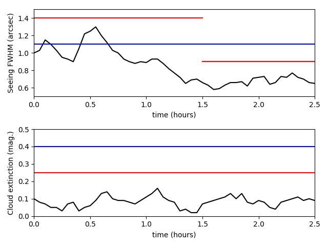
Schematic figure showing how, for an observation to be executed, the seeing and cloud extinction constraints must be less restrictive than the worst possible upcoming conditions anticipated by the queue observer (QO).
Top panel: Variable seeing FWHM is shown as a black line. The QO sets an initial maximum seeing value of 1.4 arcseconds (red line). An observation has a maximum seeing constraint of 1.1 arcseconds (blue line). After 1.5 hours, the QO finds the seeing has improved and lowers the maximum seeing to 0.9 arcseconds. The observation is initially ineligible to be scheduled because its maximum seeing constraint prevented it. After 1.5 hours, the user’s maximum seeing constraint is greater than the maximum seeing set by the queue operator and the observation becomes eligible for scheduling.
Bottom panel: A period of relatively light and stable cloud extinction. The QO correctly assesses the amount of clouds during the upcoming few hours and sets a maximum cloud extinction of 0.25 magnitudes (red line). An observation has a maximum cloud extinction constraint of 0.4 magnitudes. Because the observation's cloud extinction constraint is greater than (ie. accepting of worse than) the value set by the QO, the observation is eligible for scheduling the entire time.
- Maximum Cloud Extinction (required float; magnitudes; number ≥ 0)
Maximum cloud extinction in magnitudes is estimated during the night at the telescope and observations will be restricted to occur at times when the cloud extinction is less than or equal to a maximum value. The maximum cloud extinction set by users should be the worst (largest) acceptable value. Normally the observation will be done under less cloud extinction.
During a night of queue observing, the queue observer (QO) will calculate a schedule for upcoming observations. As part of doing that, the QO will set a value for the worst anticipated cloud extinction during the upcoming scheduled period. The cloud extinction experienced during observations should normally be less than this value. Setting a non-zero cloud extinction would permit observations on good nights when there is occasional light cirrus passing by and so that is recommended for most users.
- Maximum Airmass (optional float; range 1.0 to 2.9)
- The observatory elevation constraint for WIYN is 20 degrees. This corresponds to an airmass of 2.90. Users may set their own maximum airmass value for each target in an observation. Note that NEID's ADCs are optimized only for airmasses up to 1.7. Some degradation in RV precision might be present in observations at higher airmass. It is recommended that users set a value for maximum airmass!
- Maximum Solar Contamination (optional float; V magnitudes/arcsecond^2)
The maximum solar contamination is defined as the minimum acceptable V magnitude per square arcsecond of reflected solar flux in the background sky at the position of the target (ie twilight plus moonlight). Solar contamination is one component of the total sky background, and an error source for the high-precision stellar RV measurements done by NEID.
The effects of solar contamination are described in Roy et al. (2020):
https://ui.adsabs.harvard.edu/abs/2020AJ....159..161R/abstract
Solar contamination is not included in the current NEID Exposure Time Calculator.
Solar contamination vs. time of night is predicted for every queue target using an algorithm provided by the NEID instrument team. The algorithm is still under development and isn’t yet calibrated for WIYN.
- Minimum Distance from Moon (optional float; degrees; 0 ≤ number < 180)
- The minimum moon distance is the closest acceptable angular separation in degrees between an observation’s targets and the center of the Moon during times that the Moon is above the horizon. When the Moon is down, this constraint will not have any effect.
- Maximum Moon Illumination (optional float; 0 ≤ number ≤ 1)
- The maximum moon illumination is the highest acceptable value for the fraction of the visible side of the Moon that is in direct sunlight during times that the Moon is above the horizon. When the Moon is down, this constraint will not have any effect. Values range from 0 to 1 (new to full Moon).
Observation Timing Constraints...
Users can constrain the times over which an observation is available for scheduling with respect to various science objectives. This includes the ability: (1) to observe during very specific time intervals; (2) to request a specific number of times an observation is eligible to be done; (3) to specify observations be conducted during specific phases of a periodic ephemeris; and (4) to specify that a minimum time should elapse from a previous visit of an observation before it is repeated.
- Timing Type (required)
-
Timing type has the value 'Date-Range’' or 'Periodic'. The timing type distinguishes between observations that are tied to a user-supplied periodic ephemeris and those that are not. Some timing constraints apply only in the case of Periodic timing.
Date-Range timing is suitable for observations that are to be done one or more times. For typical NEID use, Date-Range timing will probably be the best choice for programs that are observing something other than the RV curve of an exoplanet host star with known orbital period (and even some programs wanting RV curves may find Date-Range timing is best -- see the section Observation Setup for Typical Use Cases below). For Date-Range timing, the following timing constraints apply:
- start time
- end time
- number of visits remaining
- minimum visit separation
- two visits per night
- minimum intra-night separation
Periodic type timing is suitable for observations that are to be done one or more times within one or more specific phase ranges ("phases") defined by a user's periodic ephemeris. Periodic timing was designed for users to request that spectra be taken with respect to a planetary orbital period, but is fairly general in how it is implemented. The following constraints apply:
- start time
- end time
- minimum visit separation
- two visits per night
- minimum intra-night separation
- period
- time of phase zero
- phases of interest defined by their start and end phase values
- number of visits remaining at each phase of interest
To perform periodic timing, the period, time of phase zero, and phases of interest parameters all need to be defined. In fact, entering an observation with Periodic timing without at least one row defining a phase will result in a non-functional observation.
- Start Time (UTC) (optional date-type string)
- Start time is the earliest time the observation may be scheduled. If not specified, the start of the first night of the semester is the earliest possible start time.
- End Time (UTC) (optional date-type string)
- End time is the latest time the observation may be scheduled. If not specified, the end of the last night of the semester is the latest possible end time.
- Minimum Visit Separation (required float; days; number > 0.0)
Minimum visit separation is the minimum amount of time that must elapse from the start time of one successful visit of an observation before it may be scheduled with a future start time (except in cases where two visits per night are specifically requested). Note that if minimum visit separation is set to 0 or a value smaller than the duration of the observation, and if the visits remaining is greater than 1, the observation might be executed back-to-back multiple times, using a fair amount of telescope time. Be certain you understand this and check this value! It is advised that you read the section Constraints on Separation Between Visits to understand the Minimum Visit Separation and related settings.
- Are 2 visits per night required?
It is possible to specifically request two visits of the same observation within a single night for observations of priority level 2 or higher. In these cases, a best effort will be made to either schedule and carry out two visits within a single night or nights or, if two cannot be scheduled, zero visits on a given night. If this setting is selected, a value must also be provided for the Minimum Intra-night Separation, which controls the timing of the pair of visits (Minimum Visit Separation does not pertain to this). It is advised that you read the section Constraints on Separation Between Visits to understand these types of observations.
- Minimum Intra-Night Separation (required float if 2 visits per night requested; hours)
Minimum Intra-Night Separation is the minimum amount of time that must elapse from the start time of the first visit of a required pair of visits on a single night until the second visit may be scheduled to start. This value replaces the Minimum Visit Separation for the relative timing of the pair (note too that it is in hours rather than days). It is advised that you read the section Constraints on Separation Between Visits to understand these types of observations.
- Visits Remaining (required integer; number > 0)
Visits remaining is the currently remaining number of visits requested for an observation. The visits remaining value will be automatically decremented by 1 each time an observation is done and recorded as successful by WIYN staff.
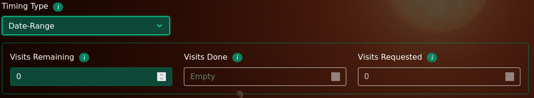
Entering values for Visits Remaining depends on the Timing Type...
For Date-Range timing, visits remaining takes a single value. Note that the observation entry page also shows values for Visits Done and Visits Requested. These are progress statuses, rather than values set directly by the user. Visits Requested indicates the most recent value set by the user in Visits Remaining, but is not decremented as observations are executed. Visits Done is the cumulative number of visits successfully completed.
For Periodic timing, there is a separate visits remaining value for each phase of interest. These are entered on a row of the entry form alongside the Phase Start and Phase End values (defined below). As with the Date Range timing, the entry page also displays values for Visits Done and Visits Requested. The "plus" sign button opens up a new row in the entry form, allowing users to enter multiple phases of interest. Once multiple phases have been defined, a red trash can icon allows users to delete unwanted phases of interest (alternatively, if Visits Remaining equals zero, a row is functionally equivalent to having been deleted).
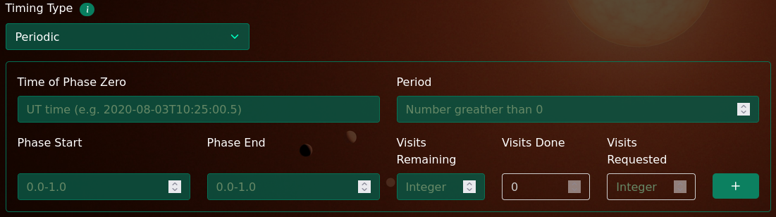
- Period (optional float; days)
The period, along with time of phase zero, defines a periodic ephemeris for an observation. This is used alongside the Time of Phase Zero parameter.
- Time of Phase Zero (optional date-type string)
- The time of phase zero is a time defining a phase value of zero in an object's periodic ephemeris. Once both period and time of phase zero are set, a phase is defined for all times throughout the semester and observations may be requested within certain ‘phases of interest’.
- Phase Start and Phase End (optional floats; 0 ≤ number ≤ 1)
Phases of interest are phase intervals within the periodic ephemeris defined by Period and Time of Phase Zero. Each phase of interest defines a set of recurring time intervals that may be considered for an observation's scheduling. The phase of interest is defined by a Phase Start and Phase End value pair. Observations may be scheduled within a phase of interest if its Visits Remaining value is > 0.
Phases are floating point values in the range 0 ≤ phase ≤ 1. With increasing time, the phase value increases until it approaches 1, at which point it becomes 0 again. A starting and ending phase defines an interval. E.g., an interval defined by (start,end) = (0.1,0.9) covers 80% of the periodic ephemeris at times excluding phase zero while an interval defined by (start,end) = (0.9,0.1) covers 20% of the periodic ephemeris at times centered around phase zero. You may enter a value of 1.0 for the end of the phase, although it is basically equivalent to 0.0. A phase value of 1.0 is mainly useful if you want to specify a phase of interest covering the entire period (set start=0 and end=1 to do this, and not the other way around!!).
Note that phases of interest may overlap and that a visit of an observation that is done at a phase that is encompassed by more than one phase of interest will be charged to the visits remaining in only one of those phases of interest.
- The actual time on target will likely be a bit shorter or longer than your request because exposures are ended when a SNR threshold or exposure time is reached and there is an integer number of exposures taken. You may describe your flexibility in this regard in the observation notes.
- If your exposure times are quite long (ie. perhaps longer than about 20 minutes), you might require even more flexibility in setting up your start_time and end_time than described above.
- Various observing constraints, set either by you or the observatory’s limiting constraints, may affect the observing availability and effectively make the observation impossible (maybe there are times within the start_time to end_time interval in which other observing constraints make it impossible to observe). The best way to check this is by using the Planning Tool, but generally you should probably avoid setting most observing constraints because you should be able to constrain the observation tightly by using just the start and end times.
- Some observers may want to start their observations "as soon as possible". For example, right at the start of the night. The best way to accomplish this would be to set the start time shortly before the beginning of the night (or half night). The Planning Tool will list the start and end times allocated for the NEID Queue on each night. If you set the start time of your observation a couple of minutes before the start of the NEID queue window, it can be scheduled to start as soon as possible on that night. Note that the observation checker will issue a warning about this, but things should work for your case!
- Certain targets (Declinations approximately 29-35 degrees North) transit close to the zenith at WIYN (within 3 degrees) and can't be observed continuously as they move close to zenith due to constraints on WIYN's tracking. These cases can be discovered using the Planning Tool. It's possible to set these observations so they appear available to the Scheduler software (ask WIYN staff to do this for you if you need it). You will, however, have to accept a period of time at night (perhaps as long as 45 minutes) when your target is unavailable. You might need to accept a long observation, like a time series during an exoplanet transit, that has a gap in coverage near zenith.
- 1. How can I observe a single target every night possible or once every few nights?
- Set up the exposure time and number of exposures (ie. exposures in each visit). Set values for the maximum seeing, cloud extinction and airmass (airmass is optional, but consider avoiding high airmass if possible). Set timing type to "Date-Range". Set visits remaining to represent your initial request for the number of times the observation should be done. Set the minimum visit separation value to 0.5 if you wish to observe once per night on every night possible. Higher values for minimum visit separation ensure the visits are more widely spaced (refer to the section Constraints on Separation Between Visits for details). Note that weather loss and competition within the queue will tend to space out your visits with longer intervals than your requested minimum. Make certain your observation is marked "active" when it is ready to go. Priority level, spectral mode and a possible request for simultaneous wavelength source are the other requirements. All settings except those set within the phase timing table may be used.
- 2. How can I observe a single host star during specific phases of a planet's orbit?
- Set up the exposure time and number of exposures (ie. exposures in each visit). Set values for the maximum seeing, cloud extinction and airmass (airmass is optional, but consider avoiding high airmass if possible). Set timing type to "Periodic". Edit the phase timing table and set the time of phase zero and period to match a planetary ephemeris. Decide on a set of orbital phases to visit and set up your initial request for the number of times you wish to observe within each phase. Use the minimum visit separation value to help space the visits out, if desired (e.g., to cover multiple orbital periods). A minimum visit separation greater than zero is also useful simply to ensure that the observation is not executed back-to-back. Make certain your observation is marked "active" when it is ready to go. Priority level, spectral mode and a possible request for simultaneous wavelength source are the other requirements. All optional settings may be used.
- 3. How can I observe a continuous sequence of exposures of some target covering a specific interval of time?
- First, refer to the section Planning Highly Time-Constrained Observations to help set up the number of exposures, start time and end time values (given your exposure time and possible SNR choice). Set timing type to "Date-Range". Set visits remaining to 1. Make certain your observation is marked "active" when it is ready to go. Priority level, spectral mode and a possible request for simultaneous wavelength source are the other requirements. For maximum cloud extinction and seeing, you might want to be open to allowing observations under some less than ideal conditions if you have limited future opportunities to repeat the observation. Generally avoid setting any other optional observing constraints because they could prevent the observation from running (ie. the setup described here controls the timing of your observation using only the start time and end time). It is useful to consider using the Planning Tool to help plan this type of observation and certainly to check out a set of observation settings.
- WIYN Cone of Avoidance
- The WIYN telescope uses an alt-az mount and cannot guide well on targets within 3 degrees of zenith. Therefore the scheduling software used by the NEID queue will not normally schedule observations of targets at times when they will move through this cone of avoidance. With the WIYN latitude of 31.958, this means, conservatively, targets between declination +28.9 and +35 (J2000). This should normally be a limitation only for the longest observations (hours long) because targets are accessible before or after they transit the meridian. If you have a long observation that must be observed over a timespan during which the target falls within the cone of avoidance, it must be specially identified and may be observed using a sequence of exposures beginning before and ending after the zenith transit, but with missing data from the time near transit. Contact Heidi and Sarah with questions about this possibility.
- Middle-of-night Calibrations and Long Observations
- Intermediate calibrations are executed in the middle of the night, sometime between 0600 and 0900 UT, for a duration of ~25 minutes. For time critical observations that need to span this entire time window, we may be able to reduce this interruption to approximately 15 minutes. In this case, please identify a time during your observation when it may be interrupted for these intermediate calibrations. This should be noted in the “Notes to Observer” field. It is generally very helpful if you note the most critical times during long observations that should not be missed. For example, ingress and egress times of a planet transit, if those are most important for your science.
- NEID Calibrations
-
- Morning and Afternoon Calibrations: These observations occur every day prior to and following observing and include darks, flats, and wavelength calibrators (i.e. arc lamps, fabry-perot etalon, laser frequency comb).
- Intermediate Calibrations: This shorter calibration sequence occurs every night that NEID is on sky near the midpoint of the night (optimized to minimize science impact when possible). A typical intermediate calibration sequence includes etalon, LFC, and flat lamp frames and takes about 25 minutes to complete.
- Bracketing Etalons: A sequence of 1 to 3 etalon frames are taken while slewing between targets during the course of the night.
- Simultaneous Etalons: For bright targets in HR mode, users may request simultaneous etalons.
- Standard Stars: One or two RV standards are observed on each NEID queue night, weather permitting, and their data are archived at NExScI with no proprietary period.
- Specialty Calibrations: Users may request special calibrations in their proposal. These specialty calibrations are the only ones whose time is charged your program's allocation.
- Notification of Data Acquisition
- An email system has been established to notify users whenever data are taken for their programs. An email should be sent out the following day.
- Data Retrieval
- The NEID pipeline and archive are housed at and maintained by the NASA Exoplanet Science Institute (NExScI). The archives can be accessed at https://neid.ipac.caltech.edu/
- NEID Calendar/Time-Critical Observations
- The WIYN telescope calendar (https://noirlab.edu/science/observing-noirlab/scheduling/mso-telescopes) indicates on which nights or half nights the NEID queue is scheduled. It is possible that NEID queue nights could be added or moved during the semester, so make sure that your observation settings illustrate any critical night required or that WIYN staff get notified of observations needing specific nights. An effort may then be made to preserve such nights in the queue schedule.
- Don't Procrastinate!
- Don’t wait until the end of the semester to add targets – many other PIs may do the same and it will be more competitive to get your observations scheduled.
- Important Instructions Not Covered By Portal Software
- Additional information that has not been conveyed within the target or observation entry pages should be sent to Heidi Schweiker and Sarah Logsdon.
- Observations for Poor Conditions
- Expanding seeing (or other) constraints may allow observations to be scheduled when others can’t. If a program has the flexibility it may be beneficial to increase these constraints to greater than the defaults (e.g. maximum seeing > 2.0 arcsec).
- Back-up Observations
- If primary targets have either already been observed or have set and there is time remaining in a program, users may want to consider adding backup targets to their program. These backup targets must retain the science goals of the original proposal.
- Consider HE Mode for Faint Targets
- Users with targets fainter than 12th magnitude may want to consider using the HE mode (with a wider diameter fiber) instead of HR mode to ensure as much stellar flux as possible is obtained.
- Faint Target Overhead
- Targets fainter than 12th magnitude may cause difficulty in acquisition and guiding, particularly in sub-optimal conditions. A larger overhead may be charged to these observations on a case-by-case basis. Good finding charts are essential for these cases.
- A semester list mode, which gives an overview of the availability of an observation night-by-night over the course of a semester.
- A single night mode, which gives a detailed breakdown of availability of an observation on one particular night (specified by UT date).
- The constraints dependent on the prior history of an observation:
- Minimum Visit Separation
- Are 2 visits per night required / Minimum Intra-night Separation
- The constraints related to unpredictable observing conditions:
- Maximum Seeing FWHM
- Maximum Cloud Extinction
- The observation status (active/inactive) or time allocations for the program
- Use the observation checker to discover and fix these!
- The possibility of invalid observation settings
- Use the observation checker to discover and fix these!
- UT Dates
- This is the UT date of the night. The dates are also links to the single night mode results.
- JD @midnight
- This is JD at midnight local time at WIYN, which is UT - 7h.
- NEID Q schedule
- This specifies which part of the night is allocated to the NEID queue. Other values refer to availability of observations only within a window of NEID operations, which runs from the end of 12-degree evening twilight to the start of 12-degree morning twilight in the case of a whole night. Half nights are stopped or started 10 minutes before or following the night center.
- Sunset (UT)
- This is approximate UT of sunset.
- Night Center (UT)
- This is the halfway time between sunset and sunrise.
- Sunrise (UT)
- This is approximate UT of sunrise.
- NEID hours
- This is the number of hours allocated for the NEID queue.
- Moon Status
- This tells if the Moon rises, sets, is up or down all night. It doesn't note when two events fall on the same night. The night runs from sunset to sunrise.
- Midnt Moon Illum
- This is the fractional illumination of the Moon at local midnight at WIYN.
- Midnt Moon Sep
- This is the separation in degrees between the target and the center of the lunar disk at local midnight at WIYN.
- Transit (UT)
- This is UT when the target transits the local meridian at WIYN.
- OK Hours
- This is the total number of hours of start availability for the observation as constrained by user constraints, telescope constraints and the hours allocated for the NEID queue. OK Hours is generally the most important bit of information from the semester list. It tells how schedulable the observation is. Note that, in some cases, the start availability is split into multiple windows of time, which may affect schedulability and that this scenario is not indicated in the semester table. A more detailed description of the start availability is available in single night mode.
- ZD OK Hours
- This is the total number of hours of start availability for the observation as constrained by limits on the target's zenith distance combined with the hours allocated for the NEID queue. Zenith distance is constrained by the maximum airmass plus a 3-degree cone of avoidance WIYN has for pointings close to the zenith.
- MoonDist OK Hours
- This is the total number of hours of start availability for the observation as constrained by the Minimum Moon Distance constraint, which is in effect when the Moon is up, combined with the hours allocated fo the NEID queue.
- MoonIllum OK Hours
- This is the total number of hours of start availability for the observation as constrained by the Maximum Moon Illumination constraint, which is in effect when the Moon is up, combined with the hours allocated fo the NEID queue.
- SC OK Hours
- This is the total number of hours of start availability for the observation as constrained by the maximum solar contamination constraint combined with the hours allocated fo the NEID queue.
- Time OK Hours
- This is the total number of hours of start availability for the observation as constrained by user timing constraints (Start Time, End Time and, for Periodic observations, phases of interest and time of phase zero) combined with the hours allocated fo the NEID queue.
- Phases available
- This column is used for Periodic observations. It lists which phases have start availability in the NEID queue hours on a particular night. The phases are those identified in the list of phases table.
- The contiguous phases numbered 2 and 3 combine together such that the start availability spans across the phase value 0.4. This means that a visit may be started at phase value 0.38, finish at phase value 0.43 and thereby span times in both phases numbered 2 and 3. The visit is credited to only one of the phase requests, however. This will apparently be phase number 3 given the midpoint of the observation at 0.405.
- The nearly contiguous phases numbered 3 and 4 are separated by enough of a gap that the start availability has a gap in the phase range 0.45 to 0.5001. This creates a gap in phase (0.475 to 0.5251) where the midpoint of an observation will never fall.
- Phase number 1 is narrower than the phase range spanned by the duration of this observation (0.04 vs. 0.05). There is no start availability for this phase given this situation and the fact that this phase is not contiguous or overlapping with another. The observation cannot be scheduled to observe this phase!
Checking/Saving the Observation and Approval
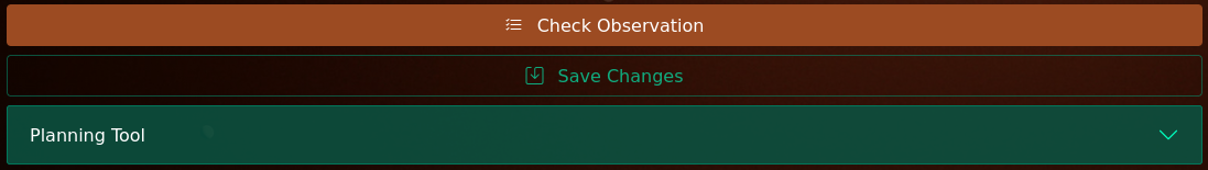
Once the observation entry form is filled out, use the Check Observation button at the bottom of the page to run the settings through a check system. This is necessary before saving the settings as an observation in the database:
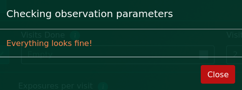
The observation checking software looks through the observation settings for problems or potential problems, such as unintended values. The results are then displayed in a pop-up window. If no issues are found, the window indicates "Everything looks fine!":
If there are problems or potential problems, these are described under a heading of Errors or Warnings:
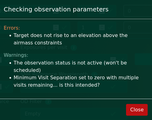
Warnings are generally less severe than Errors. Warnings are intended to help users avoid unintended problems, but might be perfectly fine for queue operations. After clicking to close the window, users can correct problems if needed. They may re-check the observation to see if warnings or errors are resolved or may submit the observation straight away using the (now enabled) Create Observation or Save Changes button (the label depends on new vs. existing observations). It is in the hands of queue users to correct their own observations and remains possible to submit a non-functional observation if the observation check goes unheeded.
Like targets, the observations go through an approval procedure by WIYN staff, which you can monitor by viewing the list of observations and the Q Status of each. A newly-submitted observation initially has a Q Status of 'Pending', then 'Approved' once approved. A Q Status of 'Requires Editing' indicates an observation that you will need to alter or confirm before it can be changed to 'Approved' and be eligible for the queue.
Note that beneath the Create Observation/Save Changes button is a 3rd widget labeled Planning Tool. This is a link to software for examining the schedulability of observations in the queue. Its use is described in detail in Appendix B: The NEID Planning Tool, but is not essential to getting started and there are other sections of this document to read first!
Editing/Copying Existing Observations
The details of your existing observations may be edited. A list of observations defined for your program may be found by selecting the ‘All Observations’ link from your Programs page. A list of observations of one particular target can be accessed from a link on the target entry page. The Obs ID link in the leftmost column of the observation list takes you to a page showing the observation details. Initially, this page is View-only.
An Edit Observation link is found at the bottom of the page:

Following this link makes the observation entry page editable, and the procedure for editing an observation matches that of entering a new one.
It is also possible to create a new observation based on a copy of an existing observation of the same target. This operation copies all of the settings from the existing observation into a new observation entry form where they may be altered before submission as a new observation. Use the Copy Observation link at the bottom of the observation entry form to do this:

Constraints on Separation Between Visits
Three settings, Minimum Visit Separation, Require 2 Visits Per Night? and Minimum Intra-night Separation provide specific control over the spacing between successive visits of the same observation. Specifically, a minimum time may be required between the start times of visits.
The simplest use of these settings involves providing a value for Minimum Visit Separation (in days) and setting the requirement of 2 Visits Per Night to 'No'. This is used for all cases other than for users that need the time sampling provided by two visits within a single night (typically meaning 2 exposures an hour or few apart).
Note that multiple visits can be scheduled within a single night without requiring two by setting the Minimum Visit Separation to a relatively small value (e.g., 0.1 days). In this case, each visit is scheduled independently and you may end up with 0, 1, 2, 3 or more visits within a given night, depending on the schedulability and competitiveness of the observation.
To avoid executing the same observation twice or more on the same night, set the minimum visit separation to 0.5 days or longer. An advantage to restricting an observation to be done only once on a given night is that the scheduling software will attempt to schedule it with its target at a relatively low airmass. In contrast, the software will consider scheduling an observation that can be observed multiple times per night in ways that permit that sampling (so possibly taking observations at a higher airmass).
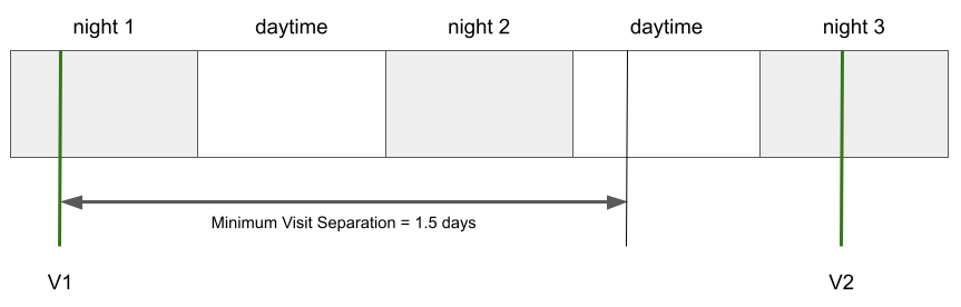
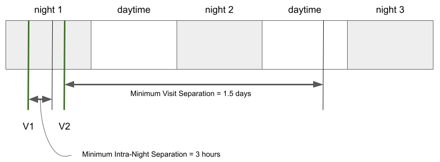
Another thing to note is that you may often want the minimum visit separation set, but with a value that ensures some other timing constraint like the day/night cycle or a periodic timing ephemeris will be the limiting constraint. For example, with a minimum visit separation of 1.5 days, an observation done on UT April 1 can be repeated on UT April 3 with the minimum visit separation having expired during the daytime preceding UT April 3. Had the minimum visit separation been set to 2 days, the constraint would have been in effect over part of the nighttime hours of UT April 3, perhaps reducing the likelihood that the observation is scheduled.
The figure below illustrates a sequence of nights on which the NEID queue could be scheduled. The time of an observation's first visit is shown by a vertical green line labeled 'V1'. A subsequent visit of the same observation is not schedulable until 1.5 days have elapsed (the Minimum Visit Separation). Since this occurs during the daytime, a second visit may be scheduled anytime during the third night as shown by another vertical green line labeled 'V2'.
Observations can be set such that visits are scheduled in pairs occurring on the same night. Since these are more difficult to schedule and have more impact on the queue, this option requires at least a priority level 2. The user must select "Yes" to the setting "Are Two Visits Per Night Required?". The spacing between visits is then controlled by both the Minimum Visit Separation and Minimum Intra-Night Separation values. Note that these values have different units (days vs. hours).
To schedule a pairs of visits, visits remaining must be at least 2 (these are separate visits in all but their relative timing constraints). Also note that each of the visits is considered to complete part of the program and that time will be charged for each single visit. Successful completion of both visits is done on a best effort basis and is not guaranteed.
The figure below illustrates a sequence of nights and the scheduling of an observation requiring 2 visits per night. The time of the observation's first visit is shown by a vertical green line labeled 'V1'. The second visit (to complete a pair) is not schedulable until 3 hours have elapsed (the Minimum Intra-Night Separation). A subsequent pair of visits may not be scheduled until the Minimum Visit Separation of 1.5 days has elapsed following the second visit. Since this occurs during the daytime, a second pair of visits may be scheduled anytime during the third night.
Observing Constraints and Scheduling
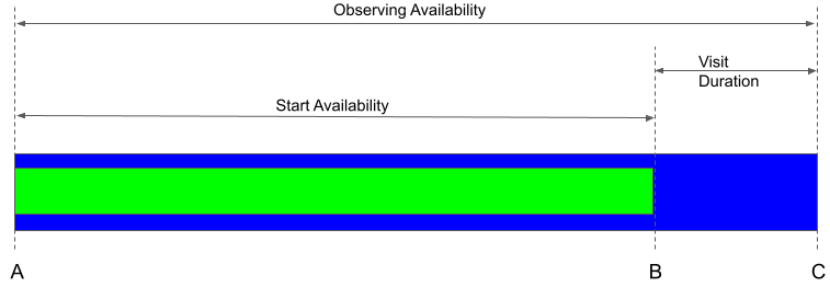
Observing availability represents the time(s) of night when all of an observation's constraints are simultaneously satisfied (excluding the unpredictable maximum seeing and cloud extinction). There may be multiple windows of observing availability on a single night. The figure below illustrates how the observing availability, the duration of a visit of an observation and the concept of start availability are interrelated. This figure represents a time axis, running from left to right.
A visit has a certain duration, which is the time between the start of its first exposure and end of its last exposure. NEID assumes that the entire visit must be scheduled so that it fits within the observing availability. In the figure, the blue bar represents a window of observing availability. The earliest time that the visit may be started (time A) is at the start of the observing availability and the latest is at time B, which precedes the end of observing availability by an amount corresponding to the visit's duration. The timespan between A and B defines a window of start availability, shown by the green bar.
NEID calculates a visit's duration based on the exposure time and number of exposures. It includes the 27s readout time between consecutive exposures. In the case of exposures that are subject to a SNR maximum, the visit duration assumed for scheduling assumes that all exposures run to their maximum exposure time.
Queue users should note that it is the duration of start availability rather than observing availability that actually affects the ease (or likelihood) of scheduling an observation. Because of this, it's best that the observing constraints are set such that there are windows of observing availability that are significantly longer than the visit duration (resulting in long windows of start availability). If not, high priority time is likely needed. In any case, a window of observing availability must be at least as long as the visit duration or it will be effectively unusable (ie. no start availability at all). Read the section Planning Highly Time-Constrained Observations for more details and advice about this issue.
Planning Highly Time-Constrained Observations
Observations must be scheduled in a queue of competing observations, and delays and inefficiencies at the telescope are unpredictable. Users planning observations of highly time-constrained events should plan with these uncertainties in mind. The scheduling software will produce a schedule of upcoming observations with each observation slated to occur at a time allowed by its constraints. A user with periodic timing should have a phase of interest that is long enough that it remains eligible after the observations get slightly out of synchronicity with the original schedule. The precision at which NEID observations may adhere to a schedule is unknown, but planning on a safety margin may be a good idea. Periodic timing constraints that result in windows of start availability at least a couple hours long should allow scheduling flexibility, but even greater availability would be optimal.
Some types of a time-constrained observation require taking a series of spectra between a start time and end time where the visit time of the observation spans (or nearly spans) the entire observing availability interval. For example, users may want to observe a star during a transit with some out-of-transit spectra taken before and after the event. The best way to define this observation is to use ‘Date-Range’ timing and specify a start time and end time resulting in an observing window a bit longer than the duration of your requested visit. There are various ways that help to define your observation but, in any case, make use of observation notes! Your notes should make it clear to the observer or WIYN staff what you want and what flexibility you have. A good approach to setting up this type of observation is to calculate the number of exposures that will cover the duration of time you wish to observe, assuming that each exposure runs for its given exposure time and that there is a 27s interval of overhead time between each exposure (ie. ignore the effects of any SNR setting you may have placed on the exposure). Request this number of exposures when setting up your observation. The duration of your observation will depend on the number of exposures (NumExp) and exposure time in seconds (Exptime), with 27s of readout between consecutive exposures:
Duration (sec) = NumExp * Exptime + (NumExp - 1) * 27s
By inverting the equation we can also find the number of exposures that produces a given visit duration. A realistic duration, of course, will be one that results in an integer number of exposures:
NumExp = (Duration (sec) + 27s)/(Exptime + 27s)
The Portal provides users with a NEID Planning Tool, which should be helpful for setting up these types of observations! For example, the Planning Tool displays the duration of the visit ("Observation duration constraint") in its output. More significantly, the Planning Tool allows a user to manipulate observation settings to quantify the availability of an observation over time.
Once you have calculated the number of exposures and exact duration (which may be different than your ideal duration), you should set the start and end time. The time span between your start time and end time should be longer than the duration calculated above. In this way, you ensure that the scheduling software considers your observation to be possible. Try to set up the start_time and end_time values so that they are at least 20 minutes longer than the duration:
end_time - start_time - Duration ≥ 20 minutes
For example, suppose you want to observe using a sequence of 300s exposures spanning a 5-hour window that is optimally between 2022-04-25T04:00:00 and 2022-04-25T09:00:00. You will find that a set of 55 exposures will have a duration of 4h59m18s with the overhead time included. If you set the start_time to 2022-04-25T03:50:00 and end_time to 2022-04-25T09:10:00, you have specified that the sequence could begin as much as 10 minutes prior to or 10 minutes after your optimal start time. This gives the observer flexibility to work the observation into the night and, we hope, enough precision for your science!
There are several things to note here:
Example Observation Setups (Typical Use Cases)
It is illustrative to describe recommended setups of observations for a few typical use cases...
Program Time Accounting
The accounting for telescope time is still in progress in 2022A. At this time, users are shown a table of hours remaining at each priority level on the Home page in the portal. Be aware that these numbers may not be the most up-to-date, but are generally correct. Users may receive the most up-to-date information via email from WIYN staff. A list of visits and time charges that are tabulated to get the hours remaining may be seen by clicking the downwards arrow link at the righthand side of this table.
Note that the Time Accounting/Program Completion link under the Programs page leads (currently) to an inactive table. This table will not have any values in it.
Appendix A: Helpful Hints
This section contains some miscellaneous items that are good for queue users to know about...
Appendix B: The NEID Planning Tool
Introduction
The NEID Planning Tool (PT) provides users with a web interface to check on the schedulability of observations given a set of observing constraints. It runs in two primary modes:
The PT can be run using links that appear at the bottom of the observation entry page. This is the case regardless of whether the fields on the observation page were filled in by querying the database for an existing observation or filled out by a human for an observation that does not (yet?) exist. In fact, it may be a good idea to view an observation in the PT before it is submitted, but after the observation has been checked. The constraints passed to the PT software are those shown on the observation entry form (with the exception of target coordinates, which correspond to a target existing in the database).
To use the PT effectively, users should understand the concepts of observing availability and start availability. These have been described in the section Observing Constraints and Scheduling. The PT reports on both observing availability and start availability. Keep in mind that for an observation to be easily (or likely) scheduled, it will probably need either long durations of start availability or high priority/time critical status.
Quick Start Advice
Observers who have relatively simple observations, which are normally of short duration without very restrictive timing constraints, may wish to use the PT to perform a brief check of their observation's schedulability. The recommended procedure would be to first run the observation checker to identify and correct problems that it identifies. Next, use the PT to look at the duration of start availability night-by-night over the semester and finally, if there are questions, examine the results for a few typical nights or those nights with unexpectedly low amounts of start availability. The PT shows a breakdown of how individual observing constraints act to limit the start availability. Users may use this information to adjust the observing constraints.
Use of the PT may be most helpful for users who have more complicated observations that they hope to have scheduled. These include time critical observations, perhaps of long duration, like a sequence of exposures timed to coincide with a planet transit. Such users may wish to dive in more deeply to ensure that their observational constraints will result in optimal scheduling. Setting up time critical observations typically involves striking the right balance of observing constraints to optimize the amount and timing of the start availability. The start availability should not be so short as to make it difficult to schedule and not too long, which can limit the accuracy of the timing of the visit. This is best done by examining availability of the observation on the specific night of interest. A start availability duration of 20 minutes is good for time critical observations such as those which coincide with an exoplanet transit.
An important thing for all users to note is that the PT does not consider how certain observation settings affect an observation's schedulability. Namely, it does not consider:
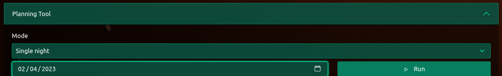
Run the PT by clicking the Planning Tool link to open up an additional "mode" selector from which you may select either "Single night" or "Semester" mode. Under semester mode, you can pick the semester of interest, although semesters too far in the future or past will not work (the PT will probably stall for a while without producing an output page). Click Run. Running the calculation for an entire semester can take some time, but subsequent runs with new settings will likely go faster. For single night mode, you will need to enter the UT date of interest (in MM/DD/YYYY format) or select it from the calendar widget linked on the right hand side of the night selector bar. Again, click Run.
Results from running the PT are displayed in a new tab and you may need to set permissions for your browser to allow this behavior on the NEID Portal.
The semester list mode displays basic target data at the top and lists the relevant observing constraints under this. The main table shows availability of the observation over the course of a semester, one night per row. The left column has the UT date and the column labeled "OK Hours" gives the total number of hours of start availability on that night. Text in the "OK Hours" column is green for emphasis. Does the amount of start availability look reasonable? If you have questions, read the detailed section below. Note that single night mode may also be run from the semester list by clicking on the UT date (leftmost column).
The single night mode results display basic target data followed by some plots, a section of ephemerides data and finally a detailed breakdown of how various observing constraints limit the availability of the observation. The top plot shows airmass and solar contamination vs. time. The bottom plot displays windows of availability as set by different observing contraints and, most importantly, the combination of all constraints ("Combined"). Green bars span the start availability. Blue bars span the observing availability. Look at the top bar that runs through the "Combined" label, if it exists. Is there start availability on this night? Is it long enough? The other bars ("Airmass/Zenith Distance", "Moon Distance" etc.) may indicate which constraints are limiting the availability. All must simultaneously overlap to allow for combined availability. For exact times of night, check out the section labeled "Combined constraint" farther down the page. If you have questions, read the more detailed description below.
Semester List Mode
The semester list output starts with a list of target name and coordinates followed by a section telling which observing constraints are being applied. One item of interest may be the Observation duration constraint, which is a calculation of the time from the start of the first exposure to the end of the last exposure. This duration ignores the possibility that a SNR constraint shortens the exposure times. It is also the time used to calculate start availability from the observing availability. For Periodic observations there is also a table that lists the phases of interest. Each entry in the table has a number in the Phase column which corresponds to a number listed in the Phases available column of the semester table.
The main semester table has a row for each night and sortable columns (ie. click on the column label to sort it then again for the reverse sort). Click on a date in the first column to examine a night in single night mode. The column values are as follows:
Single Night Mode
The single night mode applies the same constraints as semester list mode, but displays a finer level of detail.
Target information is printed at the top of the page. It is followed by a 2-panel plot:
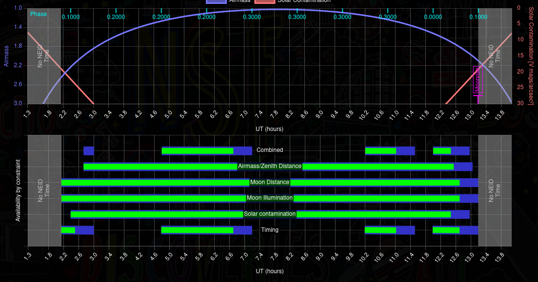
The plot above shows the availability and observing conditions predicted for a periodic observation on a dark night. The top panel displays airmass and solar contamination vs. time. This target is well positioned for this night as it transits near the night center and reaches low airmass (purple line). The pinkish line denotes solar contamination in V magnitudes per square arcsecond. The Moon is down almost all night, rising quite late at UT 13:11 at the end of the NEID queue hours. This is a dark night, so solar contamination is mainly a function of twilight and the solar contamination line drops below the plot limits to reach a very faint V=49 during the middle of the night. The plot is interactive and the actual values of airmass and solar contamination may be read for any time by moving the cursor over the plot.
The bottom panel shows how each user constraint or set of constraints limits the availability of the observation. There are 6 rows across this plot which will display times of availability using color bars, and which are labeled Combined, Airmass/Zenith Distance, Moon Distance, Moon Illumination, Solar contamination and Timing. Times along the row, but outside the coverage of the bars, are unavailable for the observation. Color coding is as follows: green bars denote start availability and blue bars denote observing availability. Greyed out areas on the plot show times outside of NEID operations. The most important component of this plot is the combined start availability (topmost green bar coinciding with the label "Combined" whenever it exists). You can see that the combined availability is the intersection of the time windows set by the other constraints on the plot. In this case, timing constraints were the most significant component limiting the combined availability.
Note that if you are checking on an observation's schedulability, look to make sure there is a green bar on the top line (alongside the Combined label). If there is no green bar, the observation cannot be scheduled!
Following the plot is a section with general ephemerides and list of observing constraints applied to the observation:
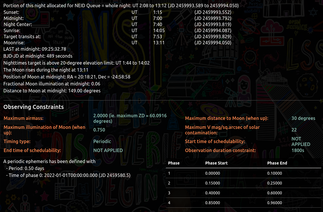
Perhaps the most important bit of information is the top line, which describes the portion of the night that is allocated for the NEID queue. This is the time that the scheduler will try to fill with planned observations. Certain time critical observations may be planned to start as soon as possible on a certain night and these should be set to be available right at the start of the NEID queue hours.
The single night mode output ends with a set of 6 sections. Each section corresponds to one constraint or a combination of constraints as well as to one of the 6 color bars in the plot. These sections list UT values describing windows of both observing availability and start availability. Other statements note when there is no availability.
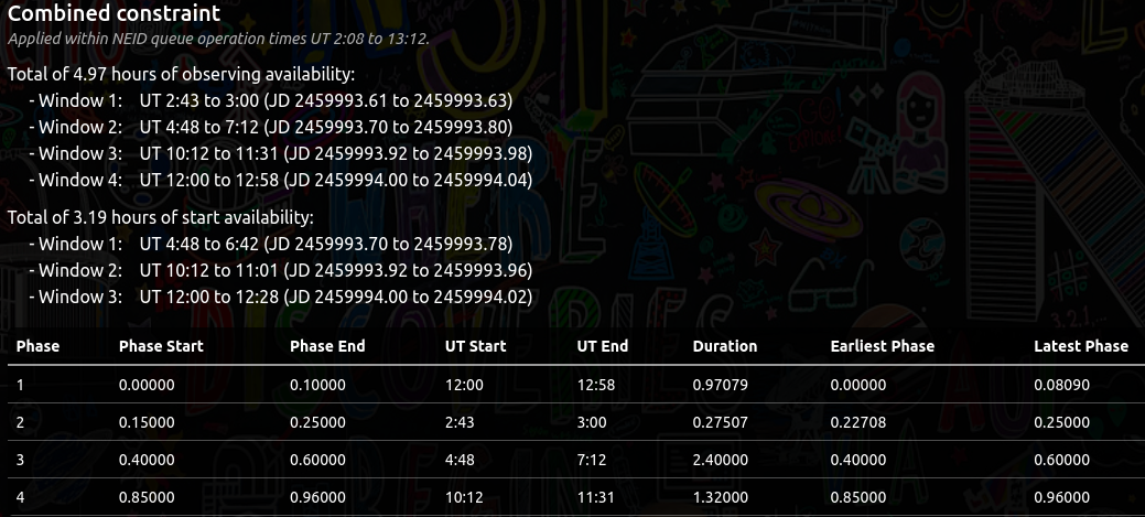
Once again, it is the combined availability, especially the combined start availability, that dictates schedulability of the observation. The first section, Combined constraint, lists the combined start availability.
For Periodic observations, a table listing availability phase-by-phase is provided in the Combined and User Timing Constraints sections. These tables show the availability broken down by phase of interest.
Using the Planning Tool for Highly Time-Constrained Observations
The section entitled Planning Highly Time-Constrained Observations describes how to set up an observation with stringent requirements on timing, especially when a visit must occur during a specific time on one night. The PT can be useful for this task as described in the example case that follows.
Suppose we wish to observe a time series of 1080-sec spectra during the transit of a hypothetical planet orbiting HD 89269. Suppose the planet has an orbital period of 6.3343134 days, a transit duration of 4.0 hours and an ephemeris with a central transit time of UT 2016-05-22T21:30:52.
We must first start by defining the target. Then we can start filling in an observation of the target. If we don't yet know which nights might be suitable for the observation, we could start out by predicting the best nights. We don't need to save the observation (it's simpler not to), but will just fill in the form to set a maximum airmass of 2, Periodic Timing Type, Time of Phase Zero to the central transit time and Period to match the orbital period. If we want to see how observable the target will be while including one hour of out-of-transit observations before the transit and one hour after, we should plan on a 6-hour long visit. These 6 hours span a phase interval of 0.03947 for the 6.33-day period (ie. (6/24)/6.3343134). Set a phase start of 0.9803 and phase end of 0.0197 to represent the series of potential visits, centered on times of predicted transits. Pick a zero duration visit by setting the exposure time to 0 and exposures per visit to 1. Without saving the observation, we can check the observation and then run the PT in semester mode (picking 2023A for our example).
The semester list shows rather limited availability this semester. We first concentrate on the Phases available column. There are 5 dates with an integer in the column, which tells us the phase we set up is available: UT 2023-02-07, 2023-02-26, 2023-04-24, 2023-05-13 and 2023-06-01. Next we look at the OK Hours column. This normally tells us how many hours of start availability there are, but since we set a zero-length visit (not 6 hours), these values really represent observing availability. For the 5 dates, the observing availability is 5.99, 1.86, 4.88, 3.57 and 2.25 hours. The 6-hour phase that covers this transit is not readily available this semester! Only on the first night (2023-02-07) are there 6 hours of observing availability. The difference between 5.99 and 6.0 hours is apparently due to some round-off errors. Click on the night of 2023-02-07 to view more details. The plot shows that the combined availability is not limited by any constraint other than our timing values, which is what we want if we wish to schedule the full observation. We could look at the details of other nights to see whether, by adjusting constraints like maximum airmass, the full observation could be scheduled then.
Note that the use of the Periodic ephemeris above assumes a constant period in UT or JD rather than BJD. Our one hour of pre-transit and post-transit time series is probably sufficient to compensate for this uncertainty, but the PT also reports BJD-JD at midnight on 2023-02-07 for this star is 494 seconds. The transit should begin 8.2 minutes earlier at WIYN than ephemeris data based on BJD predicts. We could choose slightly earlier start and end times to accommodate this offset.
If we decide to request the transit observation for the night UT 2023-02-07, we can start deciding on the number of exposures per visit, the start time and end time (and exposure time plus other constraints too, if they are flexible). The single night details for 2023-02-07 say that the 6-hour phase starts at UT 3:37 and ends at UT 9:37. If we set the start time to 2023-02-07T03:27:00 and end time to 2023-02-07T09:47:00, we set up a window of 6 hours 20 minutes for 20 minutes of flexibility in the start time. We then need to pick the number of exposures to span 6 hours. Using the equation, we estimate that (6*3600 + 27)/(1080 + 27) = 19.53 exposures will span 6 hours. We have to round off to either 19 or 20, assuming we are going to require a 1080s exposure time. Suppose we pick 20 exposures. Set the exposure time and exposures per visit in the PT. Next, for a transit-type observation, it is best if we select Date-Range as the timing type, so do that. Running the PT for 2023-02-07 now reports the observation duration as 22113s. In the Combined Constraints section, it reports a start availability of 0.19 hours (11 minutes). That's really too short! Try to get at least 0.33 hours (20 minutes) of start availability. The plot and availability listed in the Airmass/Zenith distance constraint section indicates that we can't observe any earlier with our maximum airmass constraint of 2. How about extending the end time to 10 minutes later? Perhaps we can relax the maximum airmass constraint to 2.1 and pick an earlier start time. Maybe 19 exposures would be sufficient? Would a different exposure time be okay? You can often vary multiple constraints to make the observation fit.
Appendix C: Historical Observing Conditions at WIYN
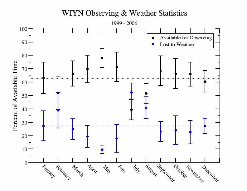
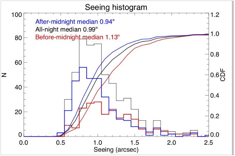
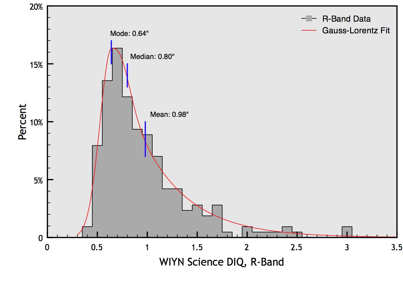
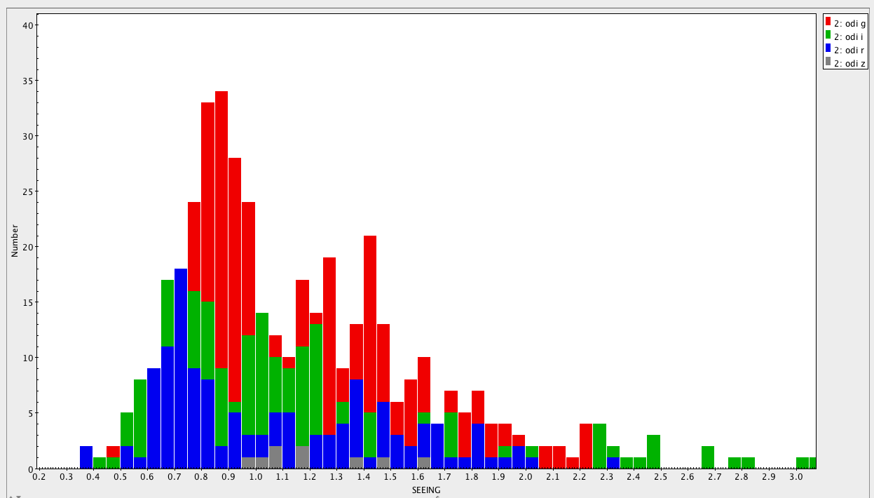
Appendix D: More About Periodic Observations
The goal behind the design of Periodic timing for NEID observations was to help users obtain RV curves for host stars of planets with known or suspected orbital period. By requesting visits at a set of specific phases, an RV curve may be sampled at the most optimal times.
When period and time of phase zero are set, all phases are mapped into times. Users can then request visits occur within certain phases of interest (range of phase defined by a starting and ending phase). Other phases can be ignored (ie. considered ineligible for scheduling). The number of visits remaining specified for each phase also controls whether a phase is considered for scheduling... a phase is ignored once its number of visits remaining drops to zero.
One thing to note is that timing constraints, including those specific to periodic observations, simply tell the NEID scheduler that certain times are eligible for visits and other times are not. There is no weighting of certain phases based upon the number of visits remaining or the fact that multiple phases might overlap at certain times.
Most users will probably not need to worry about or care about the details described below, but this is information is provided for users who are simply interested in more details or who might need intricate RV curve sampling or have difficult periodic observations with narrow phases of interest.
The behavior of overlapping phases of interest and treatment of phases of interest that are contiguous in phase coverage are described using an example below. To understand it, readers should be familiar with the concepts of observing availability and start availability for observations as discussed in the Observing Constraints and Scheduling section.
For our example, consider a Periodic observation with the following requested phases:
| Number | Phase Start | Phase End | Visits Remaining |
|---|---|---|---|
| 1 | 0.2 | 0.24 | 1 |
| 2 | 0.3 | 0.4 | 1 |
| 3 | 0.4 | 0.5 | 1 |
| 4 | 0.5001 | 0.7 | 1 |
| 5 | 0.6 | 0.8 | 1 |
| 6 | 0.9 | 0.1 | 1 |
The table contains overlapping phases numbered 4 and 5, which both include the phase range 0.6 to 0.7. It also contains two contiguous phases numbered 2 and 3 which end and begin at phase 0.4 respectively. Phases numbered 3 and 4 are nearly contiguous, separated by a gap of only 0.0001. Phase 6 is an example of a phase that wraps around the phase value of zero.
Figure 5 below shows the observing availability at each phase using a blue colored bar. The line of blue bars along the top of the plot correspond to the original set of requests where each phase has 1 visit remaining. The white space within the line of bars shows phases not requested (so not to be scheduled). For the example observation, the duration corresponds to a "delta" phase of 0.05. In a practical case, this duration in phase units depends on the observation duration in time and the Period set for the observation. For example, if Period is set to 1 day (86400s), an observation with a duration of 72 minutes will span a phase range of 0.05 (ie. 4320/86400 = 0.05). The green color in the figure indicates start availability, which is shorter than the observing availability by 0.05.
Looking at the top line of bars, there are three important things to note:
It was stated above that the gap of 0.0001 between contiguous phases numbered 3 and 4 was enough to create a gap in start availability. The way this works is that a gap in phase longer than one second is enough to create a gap in start availability. For our example with a period of 1 day, one second corresponds to a phase range of 1.16e-5. If the gap between phase numbers 3 and 4 were 0.00001, or less than one second, they would have been treated as contiguous. Note that delta phase corresponding to 1 second is expected to far exceed any roundoff errors that may be expected in the NEID software and users typing the same phase value for the end phase and start phase of two different phases can expect to end up with contiguous phases like numbers 2 and 3 in the example.
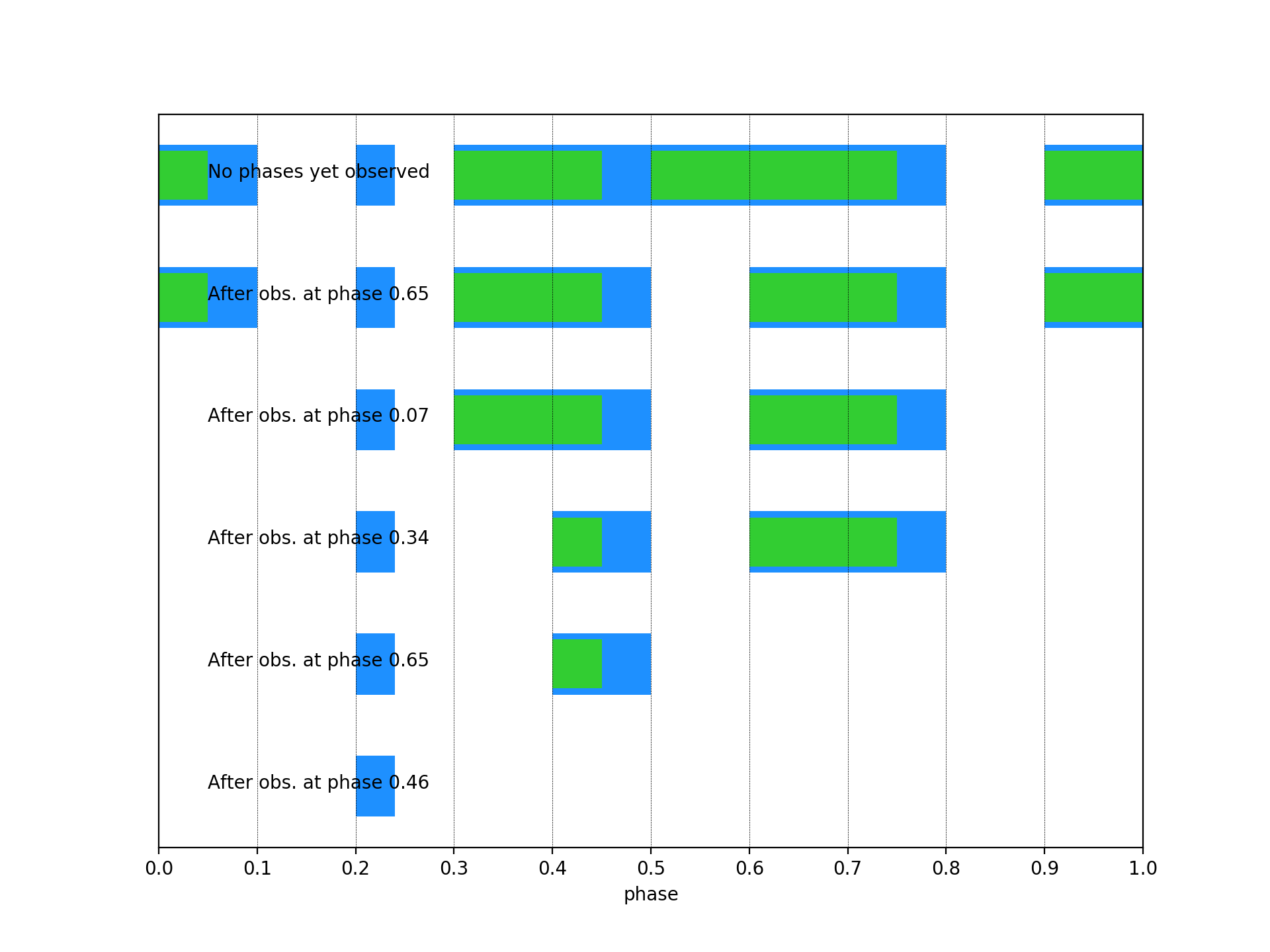
Continuing with the example periodic observation, consider how the observation’s availability changes as visits are made. Suppose the first visit is timed to fall at a phase 0.65 (phase is the midpoint in time of the visit duration, not precisely the same as the flux-weighted midpoint of the exposure(s)). This phase happens to lie where phases number 4 and 5 overlap. The effect on the observation should be considered ambiguous. One of the visits will get charged. In the example plot, this visit was charged to phase number 4 and the phase range 0.5 to 0.6 becomes unavailable. Phases around 0.65 are still available due to the request for phase number 5.
Suppose the next visit falls at a phase 0.07. This visit would have started at phase 0.045, very near the end of the start availability for phase number 6. Phases around 0 now become unavailable. After this, a visit is taken at phase 0.34, removing availability in the phase range 0.3 to 0.4. The next visit could be a repeat of a phase value seen earlier: 0.65. This time it is due to phase number 5. When that is done, the remaining start availability is rather narrow between phases 0.4 to 0.45. If that gets scheduled and observed, all available phases will be done. Only the non-functional phase number 1 remains.
Overlapping phases are probably of rather limited use for most observers, but possible. Just be aware of the ambiguities!